
An Instrument for Rapid Mesozooplankton Monitoring at Ocean Basin Scale
P.F Culverhouse1*, C Gallienne2, R Williams3 , J. Tilbury1
Affiliation
- 1Centre for Robotics & Neural Systems, Plymouth University, Plymouth PL4 8AA
- 2Plymouth Marine Laboratory, Prospect Place, Plymouth, PL1 3DH
- 3The Marine Institute, Plymouth University, Plymouth PL4 8AA
Corresponding Author
Culverhouse, P.F. Centre for Robotics & Neural Systems, Plymouth University, Plymouth PL4 8AA. Tel: +44 (0) 1752 600600; E-mail: pculverhouse@plymouth.ac.uk
Citation
Culverhouse, P.F., et al. An Instrumentfor Rapid Mesozooplankton Monitoring at Ocean Basin Scale. (2015) J Marine Biol Aquacult 1(1): 1- 11
Copy rights
© 2015 Culverhouse, P.F. This is an Open access article distributed under the terms of Creative Commons Attribution 4.0 International License.
Keywords
Mesozooplankton;Atlantic Ocean;Taxonomic;Sample
Abstract
The development and testing of a new imaging and classification system for mesozooplankton sampling over very large spatial and temporal scales is reported. The system has been evaluated on the Atlantic Meridional Transect (AMT), acquiring nearly one million images of planktonic particles over a transect of 13,500km. These images have been acquired at a flow rate of 12.5L per minute, in near-continuous underway mode from the ships seawater supply and in discrete mode using integrated vertical net haul samples. The aim of this development is to produce an instrument capable of delivering autonomously acquired and processed data on the biomass and taxonomic distribution of mesozooplankton over ocean-basin scales, in or near real-time, so that data are immediately available without the need for significant amounts of post-cruise processing and analysis. The hardware and image acquisition and processing software system implemented to support this development, together with some preliminary results from AMT21, are described. The images acquired during this Atlantic cruise comprise microplankton, mesoplankton, fish larvae and sampling artefacts (air bubbles, detritus, etc.), and were classified to one of 7 pre-defined taxonomic classes with 67% success.
Introduction
The Atlantic Meridian Transect programme (AMT[1], see Fig.1) has been conducting meridional transects of the whole Atlantic Ocean between latitudes 50°N and 50°S for 20 years (25 cruises). The Optical Plankton Recorder[2] has been used for sampling zooplankton from vertical net hauls at discrete stations, and for continuous surface underway measurements along 17 of these transects. The OPC is capable of producing rapid and robust near real-time estimates of the size-distributed biomass of mesozooplankton[3,4]. These electronic data are produced in a form permitting simple presentation as normalised biomass size spectra, from which it is possible to make estimates of secondary production process rates, for example Gomez et al[5]. In order to make such estimates, data on body size are insufficient, and some indication of taxonomic or functional grouping is necessary. No imagery is produced by the OPC, and therefore no taxonomic information is available. The development of the Line-scanning Zooplankton Analyser (LiZA) was a response to this need.
To date very few detailed taxonomic analyses have been made of the AMT samples over the twenty-five years of its operation. The difficulty with large-scale zooplankton surveys such as AMT and, for example, the Continuous Plankton Recorder[6] survey is that human expertise is required to produce a taxonomic analysis of the specimens collected. The CPR analysts currently take approximately 3 months to return results from an individual CPR tow on a ship-of-opportunity. This can be a major bottleneck in the analysis of large ecological surveys, where an inevitable trade-off has to be made between scale of survey and analysis capacity. Identification of specimens can be a subtle process, with differences between species revealed only by dissection of the specimen.
In routine analysis of plankton samples from net hauls the larger specimens such as Decapods, fish larvae, Euphausiids and Chaetognaths are counted at low magnification. To identify the smaller plankton in the sample, it is sub-sampled using a Stempel pipette or other form of sample-splitter. Usually, the analyst attempts to obtain about 200- 250 specimens per sub-sample for microscopic identification. This constitutes sparse sampling, since a net-haul could easily comprise over 12,000 specimens. By contrast, this study sets out to identify everything in a sample, but uses computer vision techniques to reduce the burden on the human expert. By doing this, the occurrences of rare specimens in a sample are noted and the respective images retained for future analysis, something both physical sub-sampling of the sample and automated machine analysis generally ignore.
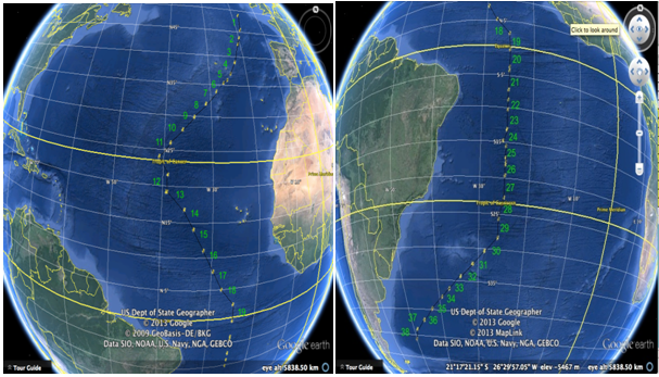
Figure 1: (a) North Atlantic AMT21 track, (b) South Atlantic track (Map courtesy of Google Maps)
In response to this bottleneck over the last 20 years instrument systems have been developed for the automated analysis and taxonomic classification of images of zooplankton acquired in situ. In this context large scale surveys have been completed using the Shadowed Image Particle Profiling Evaluation Recorder[7] (SIPPER), In situ Ichthyoplankton Imaging System[8] (ISIIS), FlowCAM[9], Underwater Vision Profiler[10](UVP), Video Plankton Recorder[11] (VPR) and ZOOVIS[12]. The Harmful Algal Bloom-buoy (HAB-buoy) system[13] was developed and successfully deployed at three sites in European waters for continuous long-term monitoring of harmful microplankton species. Images of specimens thus acquired can be pattern analysed and identified using ZooProcess[14], ZooPhytoImage[15] and Plankton Analyser[16], which are all open-source tools kits.
There are several potential difficulties associated with in situ imaging systems. Data acquisition and processing are computationally intensive tasks, and such systems often require that the process of collecting images and samples be separated from the analysis process. There is a fundamental trade-off required between (a) the need to maximise sampling volume in order to produce a statistically significant sample over an area small enough to resolve temporal and spatial variability and (b) the image resolution and computer processing demands of such large volume imaging. Few automated systems are able to analyse the entire water sample that passes through the sample chamber (see discussion of flow cell, below).
The LiZA system was developed from HAB-buoy, and together with the Plankton Image Analyser (PIA) software system (the LiZA/PIA system) has been designed and built in Plymouth to address these difficulties. The system, along with the OPC, is currently capable of producing estimates of size-distributed mesozooplankton biomass together with taxonomic or functional grouping. The categories for functional grouping were selected to permit the derivation of secondary production in the future.
Results
The LiZA system was run on AMT21 from 2nd October 2011 to 8th November 2011. For this first deployment of the system on AMT21 the automated classifier was not run in parallel with data acquisition. This was partly due to the fact that no training set could be derived until sufficient samples were gathered from all regions of the transect. It was preferred for the initial testing to run the classifier interactively post cruise with human expert intervention in order to tune and assess its performance Once a reliable training set has been assembled and refined by this process, it is intended to run the classifier in parallel with the acquisition system in order to fulfil the aim of a near real-time sampling and analysis system, with results available immediately following the end of the cruise. The expert will still be ‘in the loop’, to ensure that the rarer specimens are correctly binned and to tidy up the categories.
System Calibration
The LiZA system is used in series with the OPC, allowing inter-calibration of the two instruments in terms of particle counts and size distribution. At the beginning of each deployment, a calibration sample was run through both instruments (see Fig. 2), consisting of a number of calibration beads of 500 μm in diameter (Duke Scientific 4000 series, 500 μm ±10 μm, σ = 25.1 μm). Data acquired during sampling can also be directly compared as histograms in the same way.
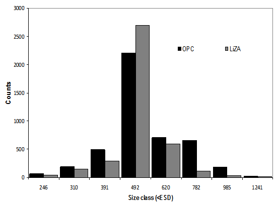
Figure 2: Inter-calibration of OPC and LiZA systems, using 500μm calibration beads.
Figure 3 shows a sample of zooplankton imagery acquired during AMT21, illustrating the typical image quality attainable. The variations in image intensity are due to specimen density differences.
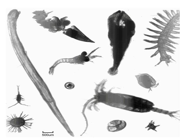
Figure 3: Montage of typical mesozooplankton images obtained by LiZA system from in-flow samples along AMT21 transect. Scale bar = 500μm.
Classifier performance
The training phase of the study using Random Forest classifier[17] revealed a 15% error. Test sets assessed subsequent to the training phase reveals error rates ranging from less than 10% to 31% with a 10-fold cross-validation. These training/test samples provided 121, 003 images, containing mesozooplankton, phytoplankton, detritus and sampling artefacts such as air bubbles. Once trained, the PIA machine sort was assessed using samples (both net hauls and in-flow) drawn from across the transect. The average sensitivity was 0.69 and precision was 0.79.
Table 1: PIA Classification % success
| Art | Blu | Cha | Cos | Det | Egg | Ost | Nau | Lco | Sca | Mic | Oit | Tri | Unc | Total N | %Correct | |
|---|---|---|---|---|---|---|---|---|---|---|---|---|---|---|---|---|
| Art | 5544 | 459 | 0 | 3 | 58 | 0 | 0 | 0 | 26 | 41 | 3 | 1 | 0 | 321 | 6456 | 85% |
| Blu | 222 | 939 | 0 | 0 | 99 | 0 | 0 | 3 | 25 | 612 | 33 | 0 | 1 | 320 | 2254 | 41.7 |
| Cha | 5 | 0 | 14 | 0 | 25 | 0 | 0 | 0 | 21 | 1 | 0 | 0 | 1 | 4 | 71 | 19.7 |
| Cos | 15 | 2 | 0 | 0 | 0 | 0 | 0 | 0 | 0 | 1 | 0 | 0 | 0 | 8 | 26 | 0 |
| Det | 52 | 103 | 2 | 0 | 791 | 0 | 0 | 15 | 114 | 467 | 7 | 6 | 4 | 28 | 1589 | 49.8 |
| Egg | 4 | 0 | 0 | 1 | 0 | 0 | 0 | 2 | 0 | 1 | 0 | 0 | 0 | 2 | 10 | 0 |
| Ost | 5 | 0 | 0 | 0 | 1 | 0 | 0 | 0 | 2 | 3 | 0 | 0 | 0 | 7 | 18 | 0 |
| Nau | 47 | 9 | 0 | 0 | 30 | 0 | 0 | 23 | 0 | 79 | 3 | 0 | 0 | 48 | 239 | 9.6 |
| Loc | 11 | 0 | 0 | 0 | 12 | 0 | 0 | 0 | 717 | 10 | 0 | 0 | 0 | 13 | 763 | 94 |
| Sca | 56 | 273 | 0 | 0 | 151 | 0 | 0 | 10 | 61 | 3918 | 46 | 14 | 0 | 676 | 5205 | 75.3 |
| Mic | 3 | 15 | 0 | 0 | 15 | 0 | 0 | 0 | 14 | 150 | 155 | 2 | 0 | 5 | 359 | 43.2 |
| Oit | 0 | 1 | 0 | 0 | 41 | 0 | 0 | 0 | 1 | 297 | 12 | 29 | 0 | 0 | 381 | 7.6 |
| Iri | 88 | 46 | 48 | 0 | 12557 | 0 | 0 | 0 | 122 | 235 | 52 | 25 | 89822 | 154 | 103149 | 87.1 |
| Unc | 84 | 25 | 0 | 0 | 96 | 0 | 0 | 3 | 49 | 107 | 17 | 2 | 4 | 96 | 483 | 19.9 |
Key: Art – artefacts; Blu – blurred; Cha – Chaetognatha; Cos – Coscinodiscus spp.; Det – detritus; Egg – eggs; Ost – Ostracoda; Nau – nauplii; Lco – large copepods; Sca – small calanoids; Mic – Microsetella norvegica; Oit – Oithona spp.; Tri – Trichodesmium; Unc – unclassified; total N = 121003
It is clear that the PIA classifier suffers from the expected under-reporting of rare classes, revealing frequent mis-labelling of crustacean eggs, Ostracoda and Chaetognaths. In addition there is frequent confusion between artefacts, blurred and unclassified when compared to the expert validated labels. The categorisation performance was low when the Random Forest classifier was asked to separate small copepoda, Oithona spp. and Microsetella norvegica, only correctly labelling the species specific categorisations 7.6% and 43.2% correctly for Oithona and Microsetella respectively. It is thought these effects are due in part to contradictions in the validated data set labelling, where the boundary between artefact and detritus, for example, is not consistently clear in the mind of the expert validator. Over a period of labelling the reference datasets, their ‘working definition’ of what constitutes a valid artefact, or blurred item or small copepod may vary. Given the size of the validated set of samples (~1 million particle images) this is not surprising. Merging Small copepoda, nauplii, Oithona spp. and Microsetella norvegica raises Small copepoda categorisation performance to 73%. Confusions between artefact and blurred and detritus results can be seen from Fig. 4.
The quality of plankton images collected in flow is good to poor: examples are shown for a variety of groups in Figs. 3, 4, 5, 6, 7, 10, 12, 15 and 18. Two additional categories were added, artefacts for air bubbles (21,728 images) and blurred that was required to cope with the poor image quality of 11,367 particles from the total of 262,972 particles in the in-flow sample of 434 cubic metres of oceanic water. This quality helped to define the selected categories. A trade-off was made between optical cell design and optical depth of field. This resulted in 4% of particle images being out of focus. This was deemed acceptable to ensure a reasonable water flow rate through the cell. However, it caused a dilemma in expert validation, since the expert sometimes made guesses as to the identity of the blurred specimen. The impact of this is discussed below.
Initially, Crustacea was selected as one of the main categories. Examination of the images in the training set showed that Copepoda dominated and Decapoda, Euphausiid etc. were far less numerous. The decision was then made to sort the Copepoda into large (> 1mm) and small (< 1mm) and then the small copepod in Calanoida, Cyclopoida and Harpacticoida. Again the quality of imagery enabled visual manual separation into genera and species such as Oithona spp. and Microsetella norvegica. Each sample took between 15 minutes and three hours to manually validate, depending upon sample size (ranging from 6,000 to 80,000 images). This resulted in categorisations that had the rarer class types removed from the abundant classes, for example eggs and Ostracoda from air bubbles and detritus. The category “small air bubbles” appears to be a catch all for all small roughly circular particles as can be seen in Fig.4 (g-h).
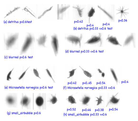
Figure 4: Examples of 2011.10.02.2018 test sample sort results. Each group of four specimen images (a, c, e and g) are annotated with the class probability. Groups b, d, f and h have individual probability annotations to highlight the uncertainty of label attribution.
Examples of the dilemma faced during interpretation of Random Forest results are shown in Fig. 5. Where the machine responses to the patterns presented were weak, several possible classifications were likely. An example from the unclassified category (Fig. 5a) shows that other possible class labels could be given to some specimens, where the classifier response was similar between two classes. Fig.5b shows a specimen labelled as blurred by the expert, and detritus by PIA. Fig. 5c shows the Random Forest Classifier taking the last label of three even probabilities and records a label of ‘unclassified’ yet equally probable was the correct label of ‘nauplii’ and an incorrect label of ‘small air bubble’. Fig.5d shows a correct label of small copepod being ascribed to the specimen, yet recorded incorrectly since the expert labelled this specimen to small calanoid. These labelling issues need resolving in a consistent manner, when equi-probable labels are presented by the classifier.
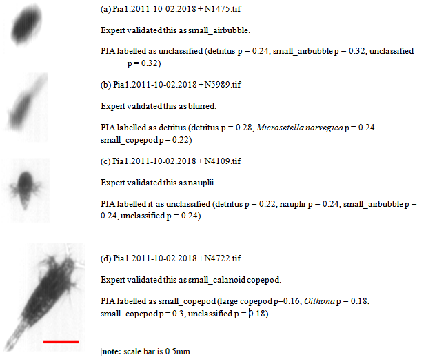
Figure 5: Detailed classification data for four specimens
An issue with image segmentation caused many Chaetognaths to be cut into several pieces where illumination striation effects appeared to separate them. The expert validator was able to recognise each as being characteristic of Chaetognatha, but PIA could not perform as well and mostly misidentified these broken up pieces as detritus. Fig. 6 gives some examples of the validator’s set of Chaetognaths from sample Pia1. 2011- 10-02.2018. Of note is specimen N2117.tif from the sample that returned similar probabilities for two of the three label categories (Chaetognatha p = 0.24, Large Copepoda p = 0.34 and Unclassified p = 0.34).
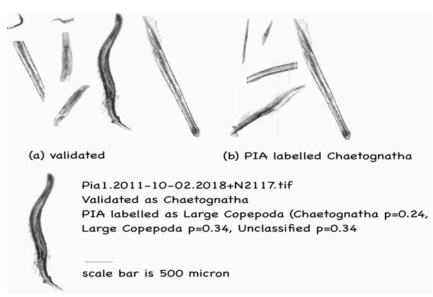
Figure 6: Chaetognatha labelling examples. Note the expert validator counted 45 partial or full specimens, whereas PIA only discovered 5, which are all shown.
Images of copepoda are shown in Fig. 7. There are many published works (for example Gallienne and Robins[3]) suggesting that Oithona spp. may be the commonest ‘small’ copepod in the ocean, yet in this 13,500 km AMT transect, sampled from a depth of 6m, the harpacticoid Microsetella norvegica (length 0.33- 0.53mm, Fig. 8) is more abundant in 28 of the 38 sampling transects, especially transects 7-21, 31°N to 4°S (Fig. 1). Oithona spp. were more abundant in the 2 most northern samples and in the 7 most southern (32° to 46°S) of the AMT transect (Fig.9).
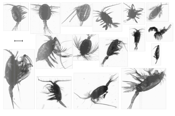
Figure 7: Images of copepoda. Scale bar 0.5 mm
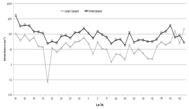
Figure 8: Large Copepoda (> 1mm) and small copepoda (< 1mm) per m³
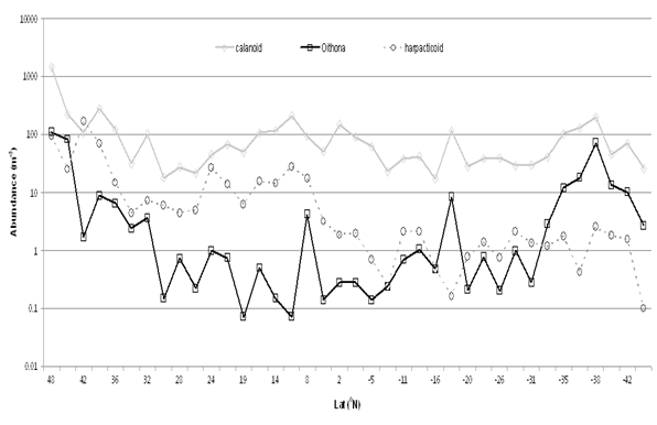
Figure 9: Calanoida, Cyclopoida (Oithona spp.) & Harpacticoida (Microsetella norvegica) distribution across the Atlantic Ocean in AM21. Numbers per m³
The small copepods (< 1mm) were present at an order of magnitude greater than the large (>1mm) copepods (Fig. 8) but the small calanoid copepods did include many other species of cyclopoid and harpacticoid (smaller Oncaea spp. Copilia spp. Corycaeus spp.), which were not discriminated in this study (Fig. 10). Other harpacticoid and the cyclopoid contribution to the small copepod category increased in the southern part of the AMT transect.
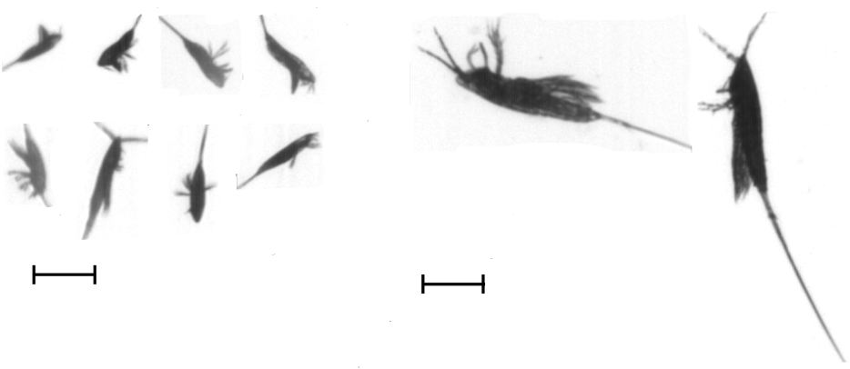
Figure 10: Selected images of Harpacticoida (a) (Microsetella norvegica) and (b) (Macrosetella gracilis). Scale bars: 0.5mm.
Ostracods were present in all transects along AMT21 (see Fig. 11), reaching a maximum in transect 38 (44° – 46°S) of 173 individuals per sample (9 cubic metres). They were rare in 12 of the 38 transects especially samples 17 -21(7° N to 7° S). The species were imaged very well with the line scan camera as seen in Fig.12; the majority observed were of the genus Conchoecia spp. The variation in grey-level is due to the differences in optical density of the specimens.
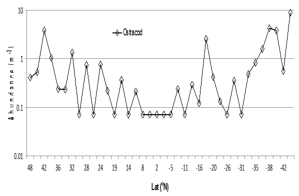
Figure 11: Ostracoda numbers per m³
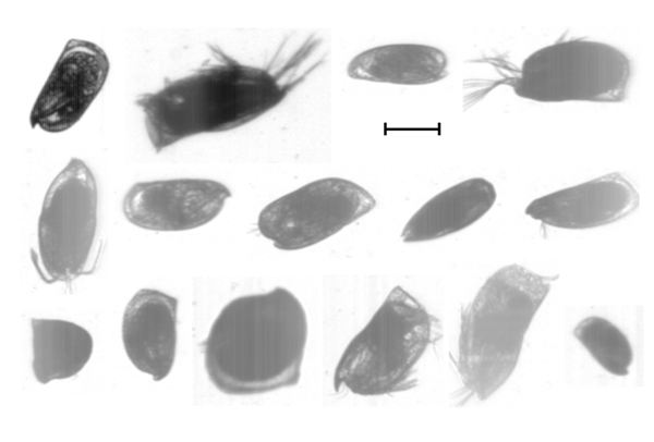
Figure 12: Images of Ostracods. Scale bar 0.5mm
Trichodesmium spp. (0.5-4 mm) is a genus of filamentous marine colonial cyanobacteria. It is the most dominant diazotroph in nutrient poor tropical and subtropical ocean waters[18] and fixes atmospheric nitrogen into ammonium. Beside single filaments, there seems to be 2 colony morphologies in our samples; they are attributed to T. thiebautii and T. erythraeum (Fig. 13).
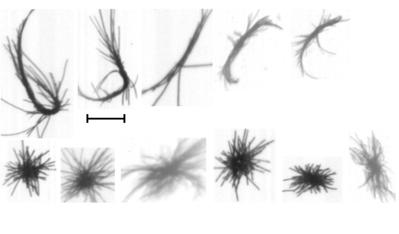
Figure 13: Image of (a) T. thiebautii (top row) and (b) T. erythraeum (bottom row) from sample 2011-10-14.0638 (23°N to 21°N) and 2011-11-05.0951 (42°N to 44°S). Scale bar 0.5 mm.
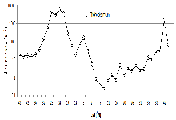
Figure 14: Trichodesmium spp. per m³.
The report by Tyrell et al[19] on analysis of AMT transects (1995- 1999) showed that Trichodesmium spp. were most abundant between 0° and 15°N but were completely absent between 5° and 30°S. These findings were based largely upon analysis of 50-100 ml samples but our samples ranged from analysis of 2.4 to 19.4 m³, which is some 48,000 to 200,000 times greater water volume analysed. This is perhaps why Trichodesmium spp. was observed throughout the whole of the north and South Atlantic Ocean on AMT 21. Our samples (Fig. 16) were taken from 6 m depth although Capone et al[20] and Letelier and Karl[21] suggest a more representative depth to sample Trichodesmium is 15 m. This suggests that this study may be underestimating the abundance. The major region of abundance of Trichodesmium filaments and colonies occurred between transects 9 to 12 (27° N 36° E to 18° N 39° E) and reached concentrations of over 5000 filaments and colonies per cubic metre (Fig. 14). This represents over 80,000 Trichodesmium imaged and counted in one transect sample. This region is further north than reported by Tyrell et al[19] as the area of maximum occurrence of Trichodesmium on the AMT track. Trichodesmium were also abundant in transect 37 (1500 filaments and colonies m³) between 42° and 44°S. The region between 5° and 17°S is of low abundance in AMT21 while Tyrell et al[19] considered it absent from 5° to 30°S. From the data collected by LiZA, sampling much larger volumes, it can be concluded that Trichodesmium is present throughout the whole of the North and South Atlantic Ocean between 48°N and 46°S and is probably ubiquitous throughout the oligotrophic oceans of the world.
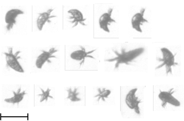
Figure 15: Selected images of copepod nauplii from sample 2011-11-05.0630 (44°S to 46°S). Scale bar: 0.5mm
Crustacea eggs and nauplii distributions (Fig.15) can be expected to vary with seasonal cycles along the AMT transect. Fig.16 shows varying, yet low, densities of both.
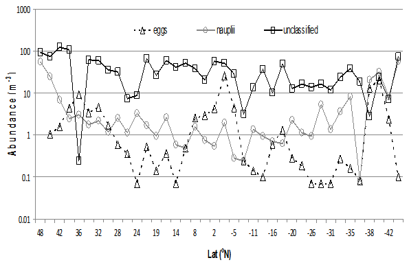
Figure 16: AMT21 distribution of eggs, nauplii and unclassified categories per m³
Detritus was distributed across the entire transect and followed a similar distribution to the ‘blurred’ category (Fig. 17). The Chaetognaths had their maximum occurrence in samples 1 (48°N – 44°N) at 46 individuals (19m-3) and 4 (38°N – 36°N) at 93 individuals (11 m-3) although occurring in low numbers throughout the AMT transect north to south.
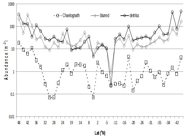
Figure 17: Distribution of blurred, Chaetognatha and detritus images across the cruise transect AMT21, per m³
Although this study was aimed at categorizing mesozooplankton along the AMT21 transect, it can be seen from the ‘unclassified’ category in Fig. 18 that the images are from plankton sizes below the normally-accepted lower size threshold of 0.2 mm, and encompasses protozoa to juvenile fish. This category contained phytoplankton (diatoms, dinoflagelates), protozoa (Acantharia, Radiolaria, Foraminifera), copepod eggs, nauplii, other mesozooplankton (Gastropoda-Creseis spp.), Crustacea (eg. Decapoda) and fish eggs and larvae.
Discussion
What is revealed by these data is a geographical distribution that broadly follows the results of previous studies of the Atlantic Ocean, but has some interesting detail, which is highlighted. The accuracy of the system will be improved in follow-up sampling and analysis on subsequent cruises, as training data sets are expanded. The acquisition and classifier systems will be run concurrently, to achieve the aim of returning from research cruises such as AMT with fully processed and analysed samples.
Compared with previous biological studies of the Atlantic Ocean, which were primarily net or bottle sampling, the near-continuous sampling of large volumes of water using LiZA, over approx. 13,500 km of ocean, indicates that some ‘presence or absence’ maps of species in the ocean may result from insufficient sampling. This appears to be the case with Trichodesmium spp. in the Atlantic Ocean, when analysed in 434 cubic metres of water.
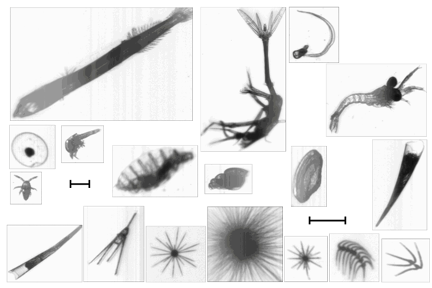
Figure 18: Images of machine-unclassified specimens. Bottom row are scaled 1:1, the remainder x 0.5. Scale bars 0.5mm.
A potential limitation of this study is that training specimens were taken from only three samples, one from North Atlantic, one from Tropical Atlantic and one South Atlantic, to construct the training dataset. These were then used to identify specimens from the entire transect: North Atlantic, tropical and South Atlantic Ocean. However, the PIA classifier returns reasonable results, although it can misrepresent rare taxa. Since the system is being assessed as a “Ferrybox” instrument it is important that ships pump induced air bubbles are handled efficiently. PIA is able to reject about 86% of these artefacts present in the water column and hence in the image sets.
In addition, there is evidence that the expert is being inconsistent in decision-making between blurred and identifiable targets on occasions. Examples of this occur with artefacts and with small copepod in relation to the amount of blurring that is acceptable to the expert in making a correct identification. It appears that mental thresholds applied to one sample may be different to those applied to another sample. In a recent study of this phenomenon by Culverhouse[22] found that plankton analysts were not consistent in their taxon labelling over a twoday period. When used as training data for machine classifiers, this human categorical labelling inconsistency causes confusion between such classes. A solution to this problem, given that performance optimisation of the classifier is on-going, is to perform a final rapid validation of the machine-classified results by an expert. Following this validation step the data appears to be consistent in the chosen categories to better than 90%. Future cruises will use a training set developed from and representative of the whole of the accumulated data set.
Conclusion
The LiZA/PIA system can process and analyse 600- 1200 litres of water per hour continuously underway and discrete net samples in a few minutes, to a specimen resolution of 100 micron. Image quality is generally good with less than 5% being blurred, and the PIA classifier is able to classify zooplankton images thus derived to one of 7 pre-defined taxonomic classes with an average of 67% success, which is good given the diversity of morphologies in each category. Results compare favourably with earlier published data for copepod abundance in the Atlantic Ocean. The effort required to complete the AMT21 data analysis to the level reported here is tractable and allows ecological data to be extracted from net hauls and in-flow pumping within a few days of the specimen images being available. This is more than a factor of ten faster than is currently possible using purely human effort. Given the compilation of a comprehensive training set for future cruises, analyses could be completed in real-time. The performance of the system is comparable to other semi-automatic imaging and identification instruments, but is the first to complete an ocean-basin scale study.
The LiZa imager captured over one million particles on the AMT21 cruise track in under-way samples and net hauls, of which 262,972 specimens were imaged underway. PIA processed and labelled all these images. The expert validator viewed all images and made a rapid re-sort to move incorrectly labelled particles to the correct bins. This took between 10 minutes and three hours to re-sort up to 120,000 specimens in a sample. It guarantees the accuracy of the labelling to an estimated 90% or better. It also ensures the rare taxa are correctly labelled, thanks to the pop-out phenomenon of human visual perception[23] in sorted samples. There was no sub-sampling of the samples at all. Everything in the 434 cubic metres of water has been coarsely sorted into seven categories. Further work will allow finer species- level discriminations of the data. The authors suggest that this is a reasonable way forward to gather detailed information at ocean basin scale using machine-assisted analysis. Until image classification can cope with rare specimen identification, with one-shot learning, this method is likely to be the best way forward for some time.
Methods: Scientific & Technological Issues
Video data is notoriously difficult to process by computer image analysis. Images that human experts find straight forward to classify can be intractable to automated image processing and classification techniques.
The LiZA in-flow system is a real-time high-speed instrument, developed from the HAB-buoy technology, capable of resolving to 100 microns (with 10 micron pixels) with flow rates up to twenty litres per minute. Samples are taken continuously for up to 22.5 hours per day from seawater drawn from the ships normal seawater supply at 6m below the surface. Daily discrete samples from vertically integrated net hauls are also processed by the LiZA system. Particle images are isolated from the water flow through the system in real-time and stored to a hard drive. These are immediately available for automated classification using the PIA classifier for near real-time image analysis and identification. Close to one million particles were acquired on AMT21 comprising microplankton, mesoplankton, fish larvae and sampling artefacts (air bubbles, detritus, etc. at a flow rate of 12.5 ± 0.49 litres per minute).
An issue of importance is the property of detritus to take on very diverse morphology - some being real body parts, or having the appearance of living organisms. This causes mistakes to be made, producing ‘false positives’ by the classifier. The magnitude of the problem depends on the amount of detritus in the water sample, since no filtering is done when operating in situ, unlike net sampling where it is normal to use a 200-micron mesh to filter out microplankton and small detritus. The higher the abundance of detritus the more likely it is to appear in other category bins. It is for this reason that we adopt the Zooscan semi-automatic methodology by Gorsky et al[14] for sample processing. This is discussed in more detail in the methods section - it allows an operator to intervene post-processing to remove obvious mistakes in machine identification. The semi-automatic methodology also allows the rarer taxa to be correctly identified by the human expert, rather than being misclassified by the machine.
System Design - Imaging System Hardware
Camera
The camera used is a Basler Sprint sp2048-70 km. This is a monochrome line-scan camera with 2048 pixels per line and a line-scanning rate of 70 kHz. Camera line rate and number of pixels, together with the flow cell dimensions and the magnification of the imaging system, determine the volume sampling rate and the resolution of the system in terms of smallest identifiable picture element (pixel). These last two parameters are conflicting (see discussion of flow cell, below) and so their chosen values must be a compromise. See Fig. 19.
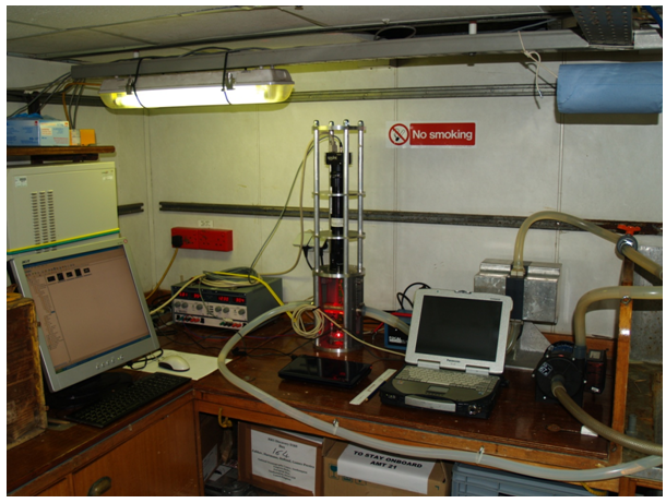
Figure 19: LiZa on board cruise AMT21, showing optics (central) and pumped water supply hoses (right).
Optics
The system uses an Infinity HDF high depth of field lens. The requirement to maximise the depth of field in order that objects are in focus across the full depth of the flow cell conflicts with the desire to maximise the resolution of the system and volume sampling rate. Again, a compromise has to be reached. In the LiZA system a working distance of 135 mm from the centre of the flow cell to the front of the lens assembly gives the required magnification of 1:1 for a maximum field of view in the object plane of 20 mm, a 10 μm resolution and a depth of field of around 16 mm.
Illumination
The LiZA imaging system flow cell is back-illuminated by a high-power light emitting diode (LED), strobe from the camera line strobe and with a duty cycle determined by a delay timer which drives the LED in pulsed mode. The LED is a Luxeon Rebel Tri-Star (MR-D0040-20T) emitting red light (626 nm) at an angle of 18°. The LED assembly consists of three such LEDs, mounted in series on a small PCB/heat sink and giving an output of 255 lm at a continuous operating current of 700 mA.
A short duty cycle, somewhat less than the camera line period, is required to prevent unwanted motion blurring as the object passes the field of view at up to 0.7 m sec-1. This requirement conflicts with the need to maximise the amount of light available during this exposure time. The line period for the camera at a line rate of 70 kHz is 14.24 μS, and the ‘on period’ for the LED is around 3μS, giving a duty cycle of approximately 20%. 3 μS represents object movement of less than half of one pixel at the proposed flow rate, so that blurring is minimised. At a 20% duty cycle the operating current can safely be increased by up to 3x without damage to the LED, giving adequate illumination over the reduced exposure period. A collimating lens in front of the LED helps to ensure that the maximum illumination reaches the object field within the flow cell, and to maintain constant illumination across the depth of the flow cell. It has been found that operating the LED in this mode using a mean current of around 1500 mA gives images of good quality and contrast without significantly shortening LED life. Typical life expectancy for the LED in this pulsed mode, used continuously day and night has been found to be greater than 60 days.
Flow Cell
The layout of the flow cell is shown in cross-section in Fig. 20, below. This cell is machined from a piece of solid brass round stock of 36 mm diameter. A hole is bored through the centre having a diameter of 25 mm. Optical windows 20 mm square and 3mm thick are set into flat recesses machined in the outside of the cell, so that their inner faces are parallel and 18.67 mm apart. The effective width of the resulting imaged area (V) is 16.7 mm. This means that in fact only a proportion of the water flowing through the system is sampled (V/[V+2D] = 0.75), and a corresponding correction factor must be applied to values for biomass concentration. It is proposed to replace the tubular flow cell with one having a rectangular cross-section to correct this, in order to achieve the potential of the system to sample all the water passing through the system.
The cross-sectional area of the imaged volume V is 312 mm². At a measured flow rate of 17.5 L/min, the linear flow through the 25 mm diameter tube is 0.59 m/sec. This linear flow increases in the reduced volume (V+2D = 418 mm²) to 0.7 m/sec. At a line scan rate of 70 kHz this yields an along flow resolution of 9.98 μm. Resolution across the flow is determined by the width of the imaged area (16.7 mm) divided by the number of pixels active across this area (1682) = 9.93 μm. Pixels in the object plane are therefore square. At other flow rates, the image will be distorted along the direction of flow (compressed or stretched). This effect was corrected at the image processing stage by assigning the correct values, based on flow rate used, to each dimension in the algorithm operating on the image.
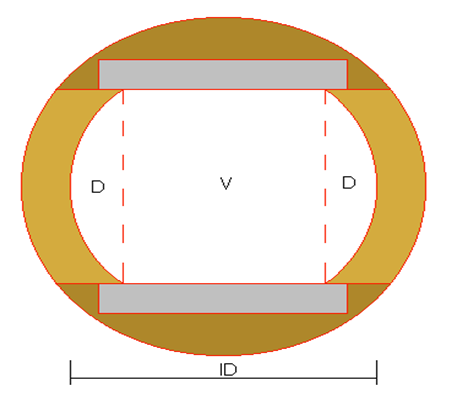
Figure 20: Cross-section of flow cell
System Throughput
The line scanning rate and the dimensions of the flow cell as determined above give an optimal volume sampling rate of 17.5 L/min, or a cubic metre of sea water in just over 57 minutes. While on-board ship the pumped seawater source could only provide 12.5L/min reliably. Generally, when in continuous sampling mode on ocean cruises such as AMT, we integrate OPC and LiZA data every hour. This gives a minimum of one cubic metre sampled, yielding sufficient numbers to produce a statistically significant size distribution up to ESD = 4mm (at least 1 present on average; Gallienne, unpublished data).
The line-scan camera works continuously and, in effect, takes one image 2048 pixels wide, by several million pixels long, depending upon sampling duration. Each pixel requires 2 bytes of storage (12-bit resolution). The system described therefore produces video data at a rate of 2048* 70,000*2 = 286.72 MB/sec. An image acquisition system capable of handling this data rate in sustained mode must be specified. A line-scan camera was chosen to ensure that the entire water column was imaged, removing the uncertainty of skipped frames, over-lapping images and gaps between images that are a serious cause for concern with normal area-scan cameras in variable flow-rate conditions. A side effect of this type of camera is that the pixel aspect ratio will change according to the water flow-rate through the imaging cell. To minimise the effect of image compression the image pre-processing accounted for this in two ways, firstly by stretching of the image to compensate the compression, and also by using logarithmic encoded parameters to encode the specimen features.
Image acquisition system
The camera is connected to an EPIX PIXCI® E4 image acquisition card mounted in a PCI Express x16 slot in a PC workstation running Windows XP. This frame grabber is capable of 700 MB/sec sustained data transfer via the PCI bus. Sufficient redundancy has therefore been built in for a possible doubling of camera line rate at a future time.
System Design – Software
Image Acquisition Software
Image acquisition and processing is achieved using a bespoke image capture system designed to process a large number of specimen images each second, with large variation in specimen concentration over time. Image acquisition by LiZA is controlled by this system, a C++ programme written and compiled by the authors using Microsoft Visual Studio 8.
Operationally, the EPIX frame grabber writes scanned lines into a circular buffer of 16 blocks of 256 scan lines. However, this means the image of a specimen can be broken up over two or more blocks. The software must recombine partial images in each block, while minimising the number of pixels it copies across memory. The EPIX frame grabber and software transfer the blocks into system RAM. The software applies a threshold boundary algorithm that visits each pixel once to create a binary mask of boundaries of each object detected, and fits a bounding rectangle. Rectangles touching the upper or lower boundary of the block are tagged as partial objects. A “stitching” algorithm is then used to combine rectangles across blocks, and pixels within completed blocks are copied out to a large circular buffer of specimen images. Another process writes the specimen images to disk. See Fig. 21 for a schematic flow diagram of the image capture process. All imaged particles are thus processed and stored to hard drive, date stamped as TIF image files.
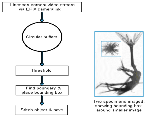
Figure 21: Image acquisition flow chart with (inset) an example of image segmentation
With this software design most pixels are only transferred from RAM to a CPU register once. Only if a pixel is part of the image of a specimen is the pixel accessed again to copy it to the circular image buffer, and eventually accessed again to write to disk. The boundary mask is small enough to fit in the processor cache memory. The rectangular data structures are small, and are reused, so also reside in cache memory. The large circular buffer of images in memory is able to smooth out fluctuations in the rate of sampling such that the system can cope for small periods of time with sampling more images than can be written to disk.
Image Analysis Software
PIA pre-processes each image, extracting numerical data from particles in the field of view following the methods described for HAB-buoy[13] and DiCANN[24] which both use the same image pre-processing method.
The resulting 134-element vector is stored in a file of such vectors, with each row unique to a specimen, one file per sample. A Random Forest classifier (from the Weka classifier toolset[25] is trained using a selected and human-identified subset of the data. Once trained, PIA is able to process a new data sample to produce a set of specimen labels, which are used to sort the sample images into one of a set of chosen categories. A Random Forest classifier[17] was chosen because it cannot be over-trained. In tests on gene classification by Statnikov et al[26] the Random Forest was out-performed by Support Vector Machines (SVM). The average performance of SVMs was 0.775 Area under ROC (AUC) and 0.860 Relative Classification Index (RCI) in binary and multi-category classification tasks, respectively. The average performance of RFs in the same tasks is 0.742 AUC and 0.803 RCI. This difference was not deemed sufficient to out-weigh the benefit of non-over-training, given unbalanced training sets.
The target categories were chosen to differentiate the images as: air streaks; air bubble large; air bubble small; blurred objects; Chaetognatha; Crustacea (copepoda >1mm); eggs; nauplii; Ostracoda; Crustacea (small copepoda < 1mm; sub-divided into Calanoida, Cyclopoida (Oithona spp.) and Harpacticoida (Microsetella norvegica, (Boeck, 1864)); filamentous cyanobacteria (Trichodesmium spp. - single strands and clusters of T. thiebautii, Gomont 1892 and T. erythraeum Ehrenberg 1830); and unclassified objects. There were insufficient images of Ostracoda, Gastropoda, Decapoda, Polychaeta, Salps, Protozoa, Dinoflagellata and many other imaged groups to make these categories useful to the training regime for the classifier. Air bubbles are present due to the nature of the water inlet and ship pump characteristics. De-bubbling was not feasible given the small size of the bubbles (< 300 micron), flow rates and the variable particle transit times caused by a de-bubbling chamber.
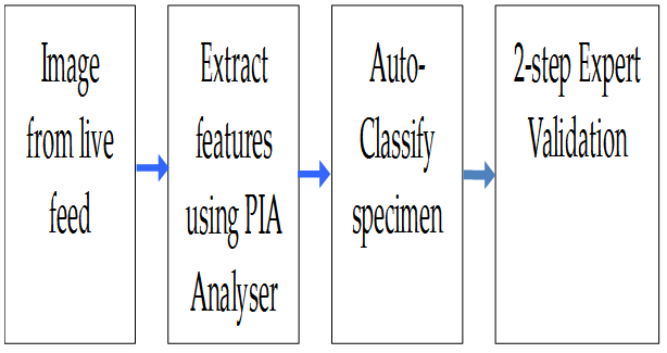
Figure 22: The image processing flow
The data processing sequence is shown in Fig. 22. Image files were UTC time stamped in the format ‘year-monthday. Time of sampling run. Item number’ and stored as uncompressed TIF files, for example 2011-11-05. 0658 + N12345.tif. This format follows the convention used by ZooPhytoImage and Zooscan.
The Random Forest Classifier was set to 50 trees, 20 parameters per tree drawn from the 134 attributes available. The training data was derived from samples 2011-10-07.0548, 2011-10-21.0648 and 2011-11-03.0516. The training set contained more than 40 examples of each target category and a total of 5,316 particles over the ten defined categories. Tests on unseen images revealed the training performance of the classifier. It gave an average of 15% training error when tested on three samples containing over 109,000 specimen images in total. This was deemed acceptable for application to all remaining samples in the study.
Results for each sample image comprise a filename, a putative category and a probability of being in that category. The probability was used to sort specimens into two folders for each category: firm and uncertain. Firm is p > 0.6, uncertain is p > 0.33 < = 0.6, unknown is p < 0.33. Items that were labelled as unknown were moved into the folder labelled “unclassified”. In development tests this technique allowed a human analyst to monitor performance by observing partially grouped sets of images. The sort is not perfect, but the high probability labels were found to be generally accurate. This segregation based upon certainty of label sped up the sorting as the low probability classifications take more time to sort, having been observed to be more diverse. The expert sorting appears to make use of the ‘pop-out’ phenomenon[23] where unusual or highly contrasting specimens appear to jump out of the field of view and become very obvious to the human. This assists the normal sequential search of images presented on a computer screen. Some net haul samples were used to assess the classifier as well, but the detail is not reported here. No class optimisation was carried out[27].
Acknowledgements: This work was carried out under the remit of Scientific Committee on Oceanic Research (SCOR) Working Group 130 for automatic plankton identification. We acknowledge the support SCOR provided to make this study possible. We wish to thank the officers and crew of the Natural Environment Research Council’s research ship RRS ‘Discovery’ for their valuable help during AMT21 cruise.
References
- 1. Robinson, C., Holligan, P., Jickells, T.D, et al. The Atlantic Meridional Transect programme (1995-2012): Foreword. (2009) Deep-Sea Res. II 56: 895- 898.
- 2. Herman, A.W. Design and calibration of a new optical plankton counter capable of sizing small zooplankton. (1992) Deep Sea Res 39(3-4): 395- 415.
- 3. Gallienne, C.P, Robins, D.B. Is Oithona the most important Copepod in the world's oceans? (2001) J. Plank. Res 23(12): 1421- 1432.
- 4. 4. Gallienne, C.P, Robins, D.B, Woodd-Walker, R.S. Abundance, distribution and size structure of zooplankton along a 20° west meridional transect of the northeast Atlantic Ocean in July. (2001) Deep Sea Res II 48(4-5): 925- 949.
- 5. Gomez, M., Martınez, I., Mayo, I., et al. Testing zooplankton secondary production models against Daphnia magna growth. (2010) ICES J Mar Sci 69(3): 421-428
- 6. Glover, R.S. The Continuous Plankton Recorder survey of the North Atlantic. (1967) Symp Zool Soc London 19:189–210.
- 7. Remsen, A., Samson, S., Hopkins, T. What you see is not what you catch: A comparison of concurrently collected net, optical plankton counter (OPC), and Shadowed Image Particle Profiling Evaluation Recorder data from the northeast Gulf of Mexico. (2004 ) Deep Sea Res I 51: 129- 151.
- 8. Cowen, R.K., Guigand, C.M. In situ Ichthyoplankton Imaging System (ISIIS): system design and preliminary results. (2008 ) Limnol Oceanogr Methods 6: 126- 132.
- 9. Sieracki, C.K., Sieracki, M.E., Yentsch, C.S. An imaging-in-flow system for automated analysis of marine microplankton. (1998) Mar Ecol Prog Ser 168: 285- 296.
- 10. Picheral, M., Guidi, L., Stemmann, L., et al. The Underwater Vision Profiler 5: an advanced instrument for high spatial resolution studies of particle size spectra and zooplankton. (2010) Limnol Oceanogr Methods 8(9): 462– 473.
- 11. Davis, C.S., Gallager, S.M., Berman, M.S., et al. The Video Plankton Recorder (VPR): Design and initial results. (1992) Arch Hydrobiol. Beih Ergebn Limnol 36: 67- 81.
- 12. 12. Bi, H., Cook, S., Yu, H., et al. Deployment of an imaging system to investigate fine-scale spatial distribution of early-life stages of the ctenophore Mnemiopsis leidyi in Chesapeake Bay. (2012) J Plank Res 1- 11.
- 13. Culverhouse, P.F., Williams, R., Simpson, R., et al. HAB-BUOY: A new instrument for monitoring HAB species. XI International Conference on Harmful Algae, Cape Town, South Africa, 15-19 November 2004. (2006) Afr J Mar Sci 28(2): 245– 250
- 14. Gorsky, G., Ohman, M.D., Picheral, M., et al. Digital zooplankton image analysis using the ZooScan integrated system. (2010) J Plank Res 32(3): 285- 303.
- 15. Bell, J.L., Hopcroft, R.R. Assessment of ZooImage as a tool for the classification of zooplankton. (2008) J Plank Res 30(12): 1351- 1367.
- 16. Hu, Q., Davis, C. Accurate Automatic Quantification of Taxa-Specific Plankton Abundance Using Dual Classification with Correction. (2006) Mar Ecol Progr Ser 306: 51- 61.
- 17. Breiman, L. Random Forests. (2001) Machine Learning 45(1): 5- 32.
- 18. Falcón, L.I., Cipriano, F.C., Chistoserdov, A.Y., et al. Diversity of diazotrophic unicellular cyanobacteria in the tropical North Atlantic Ocean. (2002) Appl Environ Microbiol 68(11): 5760-5764.
- 19. Tyrell, T., Maranon, E., Poulton, A.J., et al. Large Scale latitudinal distribution of Trichodesmium spp. in the Atlantic Ocean. (2003) J Plank Res 25(4): 405- 416.
- 20. Capone, D.G., Zehr, J., Paerl, H., et al. Trichodesmium: A globally significant marine cyanobacterium. (1997) Science 276(5316): 1221- 1229.
- 21. Letelier, R.M., Karl, D.M. Role of Trichodesmium spp. in the productivity of the subtropical North Pacific Ocean. (1996) Mar Ecol Prog Ser 133: 263- 273.
- 22. Culverhouse, P.F., MacLeod, N., Williams, R., et al. An empirical assessment of the consistency of taxonomic identifications. (2014) Mar Biol Res 10(1): 73- 84.
- 23. Treisman A. Perceptual grouping and attention in visual search for features and for objects. (1982) J Exp Psychol Hum Percept Perform 8(2): 194– 214.
- 24. Toth, L., Culverhouse, P.F. Three dimensional object categorisation from static 2D views using multiple coarse channels. (1999) Image and Vision and Computing 17: 845- 858.
- 25. Garner, S.R., Cunningham, S.J., Holmes, G., et al. Proc Machine Learning in Practice Workshop 1995 Machine Learning Conference, Tahoe City, CA, USA: 14– 21.
- 26. Statnikov, A., Wang, L., Aliferis, C.F. A comprehensive comparison of random forests and support vector machines for microarray-based cancer classification. (2008) BMC Bioinformatics 9(1): 319.
- 27. Fernandes, J.A., Irigoien, X.C., Boyra, G., et al. Optimizing the number of classes in automated zooplankton classification. (2009) J Plank Res 31(1): 19– 29.